Shared text–image embedding space with CLIP
- Source
- From the RAG & Agents Engineering course
- By
- Sourav Banerjee
- Last updated
- 9 Nov 2026
Joint embedding space
What you'll learn
- Explain how CLIP places text and images in one vector space.
- Trace a PDF through CLIP indexing: text chunks and page images in one index.
- Diagnose the two input limits that cut long chunks and small chart labels.
- Explain the modality gap, and why one shared ranking hides the right figure.
- Choose between separate quotas, one modality and a text model for text.
T6.4 built a system over text and tables. Larkspur's status reports also carry charts: monthly availability as bars, refund times by month, a server table as an image. A text-only pipeline drops them at load time, so Which month missed the 99.95% availability target? has no evidence in the index at all.
CLIP has two encoders, one for text and one for images, trained together so that an image and a caption describing it land close in the same vector space (Radford et al., Learning Transferable Visual Models From Natural Language Supervision, 2021). That shared space is a joint embedding space: a text question can retrieve an image directly. With openai/clip-vit-base-patch32, notebook 01a's model, both encoders end in a 512-dimension vector. The notebook normalises each to unit length, so a dot product is a cosine.
Here is what 01a does with a PDF:
| Step | Text | Images |
|---|---|---|
| Extract | Each page's text, split into 500-character chunks with 100 of overlap | Every embedded image on the page |
| Embed | CLIP's text encoder | CLIP's image encoder |
| Store | One FAISS index for both, ranked by L2 distance, which on unit vectors orders results like cosine | Same index; each image is a stub document marked as an image, with the image kept as base64 for the answer model |
| Answer | The question goes through the text encoder; the top 5 come back | Retrieved images go to a vision-capable chat model as image parts of one message (T3.2 covers that format) |
Table 1: CLIP indexing and retrieval in 01a.
Two input limits
Both encoders have hard input limits, and both matter for documents:
| Limit | What CLIP does | What a document loses |
|---|---|---|
| Text stops at 77 tokens | Truncates the rest, without a warning | 01a's 500-character chunks run past 77: split the same way, page 2 of the Attention paper gives 11 chunks of 81 to 116 CLIP tokens, and even the sample PDF's 365-character page is 79 |
| Images become 224 by 224 | Scales the shortest side to 224 and crops the centre square, then reads 7 by 7 patches of 32 pixels | A 400 by 300 chart becomes 299 by 224 and loses about a quarter of its width; small axis labels and printed values rarely survive |
Table 2: CLIP's input limits and what they cut.
CLIP was trained to match images with short captions, so a long paragraph is outside what it learned. We call the first row the silent truncation: the tail of every chunk is gone, and nothing in the output says so.
01a's own sample cannot show a failure. Its PDF holds one 365-character text chunk and one 400 by 300 image of three unlabelled bars, so the index has two items and k = 5 returns both for any question. The scores still show the pattern of the next section: for What does the chart on page 1 show about revenue trends? the text chunk scores 0.651 and the chart 0.270.
One ranking, two modalities
The interactive chart retrieval lab indexes three Larkspur status-report pages with 01a's own embedding functions: six text chunks and three figure images in one index, nine items. The scores split into two bands:
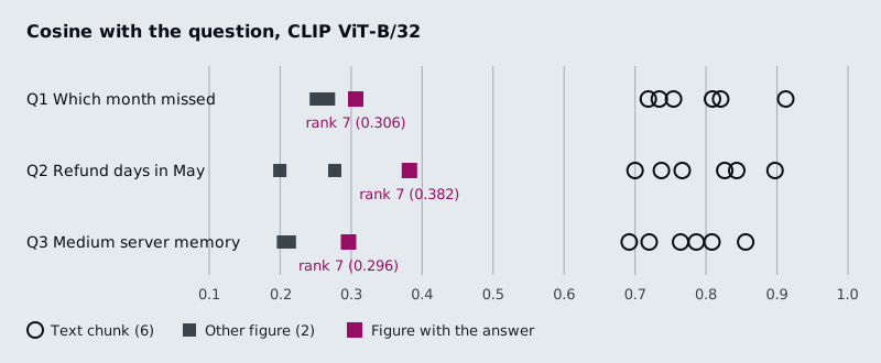
Figure 1: CLIP scores on the lab pages. Every text chunk outscores every image.
Every text chunk scores between 0.692 and 0.912 against every question; every image scores between 0.200 and 0.382. Liang et al. measured this split across contrastive models and named it the modality gap (Mind the Gap, NeurIPS 2022).
Inside the image band, CLIP does its job. For each question, the image with the answer is the best image:
| Question | Answer figure | Score | Best other image | Answer figure's rank in the shared index |
|---|---|---|---|---|
| Which month missed the 99.95% availability target? | Figure 1 | 0.306 | 0.268 | 7 of 9 |
| How many business days did a refund take in May? | Figure 2 | 0.382 | 0.277 | 7 of 9 |
| How much memory does the Medium server have? | Table 1 | 0.296 | 0.213 | 7 of 9 |
Table 3: The answer figure is the best image and the seventh item (the module's chart retrieval lab).
In the shared ranking that does not help. Each answer figure sits behind all six text chunks, so 01a's k = 5 sends five text chunks and no image, and the model never sees a bar. It takes k = 7 to reach the figure, and then the model reads six chunks of text to use one picture. We call this the buried figure.
Key distinction: CLIP's scores are comparable within a modality and not across modalities. A figure at 0.306 is a strong image match; a text chunk at 0.692 may be a weak text match.
Choosing around the gap
Since scores from different modalities are not comparable, do not rank them together:
| Option | How | Trade-off |
|---|---|---|
| Separate quotas | Search text and images separately; send the top text chunks plus the top image | On the lab pages the top-1 image is the answer figure for all three questions; costs one more search |
| One modality | Turn figures into text (lesson 2 of T6.5) or text into page images (lesson 3 of T6.5) | Every score comes from one comparison; captioning costs a vision call per image, page images cost a large index |
| A text model for text | Embed chunks with a text embedding model (T5.4); keep CLIP for image search | Fixes the 77-token cut; the two searches still need separate quotas |
Table 4: Three ways around the modality gap.
In practice: Larkspur's status reports
- Index figures and text separately, with a text embedding model for the chunks and CLIP for the images.
- Send a quota: the top 4 text chunks and the top 1 image.
- Check figure resolution: a chart whose values are small printed labels may need captioning (lesson 2 of T6.5) rather than CLIP.
- Add a chart-only golden question per report, such as the availability month, so a buried figure shows up as a miss.
Lesson 2 of T6.5 removes the gap the other way: it turns every figure into text before indexing.
Run the notebooks
The code for this lesson is in these notebooks. Colab runs one in your browser: install the packages its first cell imports and set the API keys it reads. To run every notebook as written, clone the repository and use its uv environment.
| Notebook | GitHub | Colab |
|---|---|---|
| Multimodal RAG with clip | Open on GitHub | Open in Colab |
Key Takeaways
- CLIP puts text and images in one 512-dimension space, but its text side stops at 77 tokens (the silent truncation) and its image side crops to 224 by 224, so long chunks and small chart labels are lost.
- Text and image scores sit in separate bands (0.692 to 0.912 against 0.200 to 0.382 on the lab pages). In one shared ranking the right figure falls behind every text chunk (the buried figure).
- Do not rank modalities together: use separate quotas, convert everything to one modality, or embed text with a text model.
Check yourself
1. Notebook 01a splits pages into 500-character chunks before embedding them with CLIP. What happens to each chunk?
CLIP's text encoder stops at 77 tokens and truncates the rest without a warning. Split that way, page 2 of the Attention paper gives chunks of 81 to 116 CLIP tokens, so every chunk loses its tail. CLIP was trained on short captions, so a text embedding model is the better retriever for paragraphs.
2. For the availability question, Figure 1 is the best-scoring image at 0.306, yet with k = 5 the model never sees it. Why?
The modality gap: every text chunk scores between 0.692 and 0.912 and every image between 0.200 and 0.382, so in one shared ranking all six text chunks come before any image. Figure 1 ranks 7th of 9, and k = 5 sends only text. It is the buried figure.
3. How would you change the retrieval so the answer figure reaches the model for all three lab questions?
Search text and images separately and send a quota, such as the top text chunks plus the top image: on the lab pages the top-1 image is the answer figure for all three questions. Alternatively convert everything to one modality, by captioning figures (20.2) or retrieving page images (20.3).